github-showcase-page-abc123
github-showcase-page-abc123 created by GitHub Classroom
Building a Competitive National Football Team

Group Members
- Lenny Han - z5258272
- Thomas Jiang - z5255865
- Zekai (Eric) Kuang - z5256982
- Celina Mak - z5255598
Table of Contents
Table of Contents
Overview
This landing page showcases the methodology behind the construction of Rarita’s national football team using statistical models and analyses the impact of a competitive team on the country’s economy. Here, we outline several key considerations in our team selection including data cleaning, assumptions, methodology, economic impacts and risks and limitations.
Project Objectives
 The objectives of this project included:
- Ranking within Football and Sporting Association’s (FSA) top ten members within the next five years and,
- Having a high probability of winning an FSA championship within the next ten years.
By developing Rarita’s national football brand, the overarching objective was to achieve positive economic impacts for the country over the next 10 years such as GDP growth.
Data Cleaning
R was used to firstly clean/standardise the raw datasets.
League defending, passing, shooting, salary, and goalkeeping statistics were imported from the case data in Excel: 2022-student-research-case-study-player-data.xlsx
#Load packages
install.packages("tidyverse")
library(tidyverse)

#Load data
ld <- read.csv("ld.csv",header=T,stringsAsFactors=T)
lg <- read.csv("lg.csv",header=T,stringsAsFactors=T)
lp <- read.csv("lp.csv",header=T,stringsAsFactors=T)
ls <- read.csv("ls.csv",header=T,stringsAsFactors=T)

sal20 <- read.csv("sal20.csv",header=T,stringsAsFactors = T)
sal21 <- read.csv("sal21.csv",header=T,stringsAsFactors = T)

#Remove duplicated data points
sal20 <- sal20[!duplicated(sal20),]
sal21 <- sal21[!duplicated(sal21),]
The data was separated by the associated year (2020 and 2021).
ld20 <- ld %>% filter(Year==2020)
lg20 <- lg %>% filter(Year==2020)
lp20 <- lp %>% filter(Year==2020)
ls20 <- ls %>% filter(Year==2020)

ld21 <- ld %>% filter(Year==2021)
lg21 <- lg %>% filter(Year==2021)
lp21 <- lp %>% filter(Year==2021)
ls21 <- ls %>% filter(Year==2021)
Defending, shooting, passing, and salary data were then joined to create a single dataset. Goalkeeping data was separated due to the different set of measured statistics.
ldp20 <- left_join(ld20,lp20,by=c("Player","Nation","Pos","Squad","League","Year"))
ldps20 <- left_join(ldp20,ls20,by=c("Player","Nation","Pos","Squad","League","Year"))
ldpss20 <- left_join(ldps20,sal20,by=c("Player"))
lgs20 <- left_join(lg20,sal20,by=c("Player"))

ldp21 <- left_join(ld21,lp21,by=c("Player","Nation","Pos","Squad","League","Year"))
ldps21 <- left_join(ldp21,ls21,by=c("Player","Nation","Pos","Squad","League","Year"))
ldpss21 <- left_join(ldps21,sal21,by=c("Player"))
lgs21 <- left_join(lg21,sal21,by=c("Player"))
N/A and negative data were set to equal 0 to avoid data issues in later modelling steps.
ldpss <- union_all(ldpss20, ldpss21)
ldpss[is.na(ldpss)] <- 0
ldpss[is.negative(ldpss)] <- 0
Assumptions
Team Selection
| Factor | Assumption |
|---|---|
| Salary | Player salaries were used as a proxy for their overall ability, with more skilled players being paid higher salaries. |
| Salary Growth | In line with Rarita’s inflation rates. |
| Inflation Rates | Projected using a moving average of inflation rates from the preceding 5 years. |
| Tournament Performance | Tournament performance is positively correlated with economic impact. |
| Loan Provisions | The loan fee is charged recurringly on an annual basis. |
Economic Impact
| Factor | Assumption |
|---|---|
| Inflation | Projected from 2021-31 using a 5-year moving average with projected rates of 2.5-3% over the period, which is in-line with Rarita’s historical inflation trends. |
| Discount Rate | Set as 1.9%, the 10-year treasury yield as of 2021 for Rarita. |
| Commercial Revenue | A mix of inflation and social media growth was used to project commercial revenue. |
| Broadcast Revenue | Average annual growth over 2016-19 was used to estimate long-term growth. |
| Staff Expenses | Estimated using existing per capital staff expenses and salary of constructed team. Projected under best-estimate of inflation for future periods. |
| Matchday Revenue and Other Expenses | Projected using estimated inflation. |
| Social Media Growth | Best estimate of 5% annual growth rate using baseline scenario of Rarita’s tournament performance. |
| GDP Growth | Baseline economic scenario projected using linear regression model on Healthcare Spending, Savings Rate and Population Density. |
Team Selection Methodology
Feature Selection
A random forest model was developed to predict the salaries of players using their measured statistics to identify high performing players and select the most competitive team for Rarita.
library(gbm)
library(randomForest)

ball <- read.csv('ldpssmerged.csv', header = TRUE)
Age and league treated as factors in model.
ball$Player <- NULL
ball$Age <- as.factor(ball$Age)
ball$League <- as.factor(ball$League)

ball[is.na(ball)] <- 0

ball_gk <- ball %>% filter(str_detect(ball$Pos, "GK"))
Dataset portioned into training and test set with an 80:20 split.
set.seed(1)
training_set <- sample(length(ball$Salary), 0.8*length(ball$Salary))
train <- ball[training_set, ]
test <- ball[-training_set, ]
Random Forest model for forwards, midfielders, and defenders fit using training and testing sets.
#Model fitting on training set
p <- length(ball) - 1     #Number of predictors in the data set
m <- round(sqrt(p))
rf_fit <- randomForest(as.numeric(Salary) ~ ., data = train, mtry = m, importance = TRUE)
varImpPlot(rf_fit)

#Re-run random forest model after selecting most important variables
rf_fit1 <- randomForest(as.numeric(Salary) ~ League + Pressures.Def.3rd + Pressures.Mid.3rd + Pressures.Att.3rd + Int + Clr + Long.Att + KP + Standard.Sh.90 + Standard.SoT.90 + Expected.npxG, data = train, mtry = m, importance = TRUE)
varImpPlot(rf_fit1)

#Model fitting on testing set
p <- length(train) - 1     #Number of predictors in the data set
m <- round(sqrt(p))
rf_fit_test <- randomForest(as.numeric(Salary) ~ ., data = test, mtry = m, importance = TRUE)

#Re-run random forest model after selecting most important variables
rf_fit1_test <- randomForest(as.numeric(Salary) ~ League + Pressures.Def.3rd + Pressures.Mid.3rd + Pressures.Att.3rd + Int + Clr + Long.Att + KP + Standard.Sh.90 + Standard.SoT.90 + Expected.npxG, data = test, mtry = m, importance = TRUE)
varImpPlot(rf_fit1_test)
A separate random forest model was fit for goalkeepers due to varying measured statistics.
p_gk <- length(ball_gk) - 1     #Number of predictors in the data set
m_gk <- round(sqrt(p_gk))
rf_fit_gk <- randomForest(as.numeric(Salary) ~ ., data = ball_gk, mtry = m_gk, importance = TRUE, na.action = na.roughfix)
varImpPlot(rf_fit_gk)
GBM was also fit, with results compared to Random Forest.
#For forwards, midfielders and defenders
b_fit <- gbm(Salary ~ ., data = train, distribution = 'gaussian', n.trees = 5000, interaction.depth = 3, shrinkage = 0.01, cv.folds = 10)
b_prob <- predict(b_fit, newdata= test, n.trees = which.min(b_fit$cv.error))
b_comparison <- abs(b_prob - as.numeric(test$Salary))

#For goalkeepers
b_fit_gk <- gbm(Salary ~ ., data = ball_gk, distribution = 'gaussian', n.trees = 5000, interaction.depth = 3, shrinkage = 0.01, cv.folds = 10)
b_prob_gk <- predict(b_fit_gk, newdata= ball_gk, n.trees = which.min(b_fit$cv.error))
b_comparison_gk <- abs(b_prob_gk - as.numeric(test$Salary))
It was found that Random Forest performed similarly to GBM, whereby due to the potential for GBMs to overfit, the Random Forest model was chosen for feature selection in identifying top performing players. This model fitting process was repeated by excluding the least important and unstandardised variables (such as aggregated statistics rather than per 90-minute statistics) to prevent overfitting and collinearity amongst predictors.
The most significant predictors were determined by setting a lower bound for its contribution to percentage of variance explained, predictors below this threshold were removed. This ultimately led us to a Random Forest model that only included the most significant predictors of player salary, which were then used to build our player metric.
Player Metrics
Forwards, Midfielders and Defenders Metric
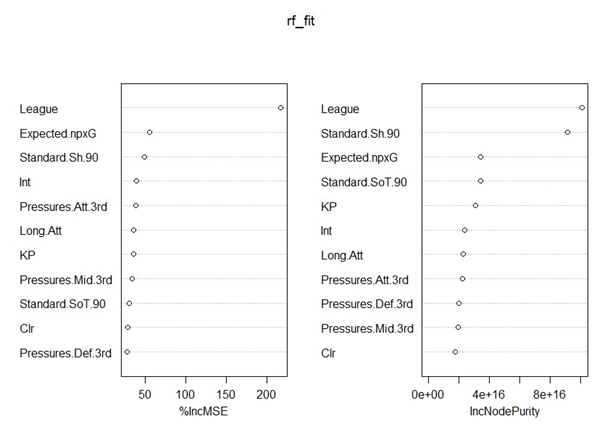
Based on the variable importance results above, the following player statistics were chosen for forwards, midfielders, and defenders:
| Statistic | Definition | Variable Importance Weighting |
|---|---|---|
| Expected.npxG | Non-penalty expected goals | 0.1729 |
| Standard.Sh.90 | Shots total per 90 minutes | 0.1378 |
| KP | Passes leading to a shot | 0.1155 |
| Long.Att | Passes >30 yards attempted | 0.0755 |
| Int | Interceptions | 0.1015 |
| Pressures.Def.3rd | Pressure applied to opponent in the defensive 1/3 | 0.0533 |
| Standard.SoT.90 | Shots on target per 90 minutes | 0.0937 |
| Pressures.Att.3rd | Pressure applied to opponent in the attacking 1/3 | 0.1065 |
| Clr | Clearances | 0.0719 |
| Pressures.Mid.3rd | Pressure applied to opponent in the middle 1/3 | 0.0714 |
Goalkeeper Metric
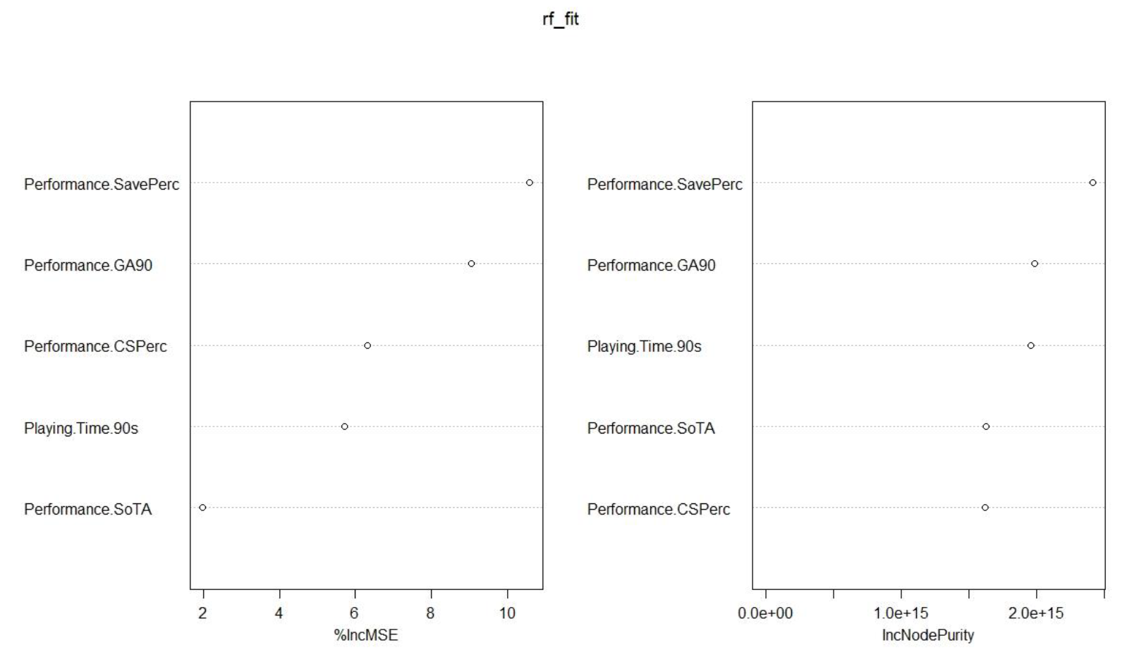
Based on the variable importance results above, the following player statistics were chosen for goalkeepers:
| Statistic | Definition | Variable Importance Weighting |
|---|---|---|
| PlayingTime90s | Minutes played per 90 minutes | 0.1190 |
| PerformanceGA90 | Goals against per 90 minutes | 0.1988 |
| PerformanceSoTA | Shots on target against | 0.1269 |
| PerformanceSavePerc | Shots saved as a % of shots on target against | 0.4046 |
| PerformanceCSPerc | % Match with clean sheet | 0.1508 |
A weighted average of the selected statistics was the final metric used to evaluate the players. The weights were formulated as a proportion of their respective variance importance figures in the random forest model. For players exhibiting similar metric figures, the cheaper player was chosen as they provided more “value” on a per dollar basis. The National Football Team selected can be viewed below.
Comparison Against Competitors
An equivalent team metric was calculated for the selected team as well as the top-10 nations in the 2021 Tournament.
![]()
Higher ranking teams typically exhibited larger metric scores, confirming the metric’s validity and accuracy in evaluating player and overall team performance. The selected team produced an average metric of 1.271 with a standard deviation of 0.323. Using a normal approximation, this yielded a lower bound of 0.638 for a 95% confidence interval, and a lower bound of 0.441 for a 99% confidence interval. In comparison to the participating nations in the 2021 Tournament, the selected team yielded a 95.818% and a 9.510% probability of a top-5 and first-place finish respectively. Althought the chosen metric may not accurately project the future performance of all teams, the probability measures strongly suggests Rarita’s team can consistently outperform the tournament participants based on their 2021 Tournament performance. Thus, the “competitive” criteria of the objective can be satisfied.
National Football Team Selected
| Player | Nation |
|---|---|
| Y. Rabinovitch | Western Niasland |
| G. Katumba | Biarizea |
| M. Nkhata | People’s Land of Maneau |
| M. Rashid | Sobianitedrucy |
| C. Kakayi | Dosqaly |
| S. Rizzo | Sobianitedrucy |
| X. Takagi | Rarita |
| V. It | Mico |
| O. Nakisige | Reugha |
| A. Fekete | Byasier Pujan |
| M. Kabiru | Sobianitedrucy |
| F. Among | Biarizea |
| D. Makumbi | Rarita |
| K. Mawanda | Varijitri Isles |
| P. Anderson | Esia |
| J. Yeo | Dosqaly |
| I. Tabu | Rarita |
| K. Kazlo | Rarita |
| Z. Nyamahunge | Rarita |
| F. Ithungu | Rarita |
Implementation Plan
An implementation plan was created to facilitate ongoing monitoring and respond quickly to changing circumstances and emerging risks which will ensure a competitive football team. This was created as an annual framework to monitor progress over the next 10 years, as illustrated below.
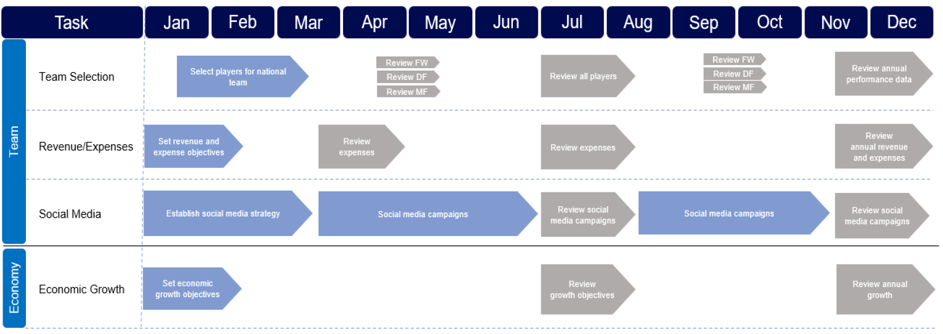
The constructed implementation timeline has regular monitoring efforts and flexibility to adapt to changing circumstances that could otherwise lead to adverse effects for the team.
Economic Impacts
GDP Projections
Rarita’s GDP growth was projected over the 2021-31 period using a linear regression model (GDP Projection.xlsx), with the predictors:
- Population density
- Healthcare spending per capita
- Household savings rate
The model was constructed using the provided economic and sociodemographic data for Rarita from 2011-19, resulting in an adjusted R-Squared metric of 0.898 and all variables being significant and jointly significant at a 5% p-value. Each of the predictors were then projected separately over the forecasting period using their respective historical average growth rates. GDP growth was then estimated using these forecasted values for the predictors.
Net Revenue Projections and Expected NPV
Using the best estimates of economic and expense/revenue assumptions set out above, a model projecting the football revenues and expenses that Rarita will face over 2021-31 was developed under the expectation that the national football team constructed would remain competitive throughout the period.
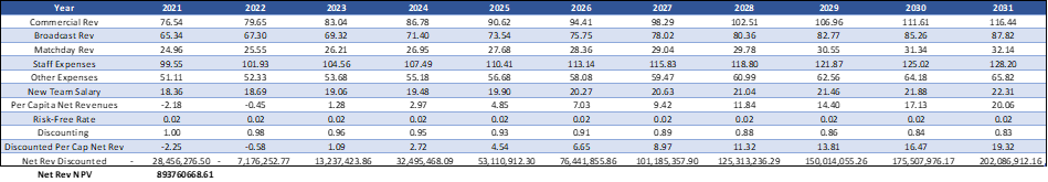
The Net Present Value (NPV) generated by the selected team over the 10-year period is expected to be 74.87 Doubloons per capita, or a total of 893.77 million Doubloons. A large outlay of cash is expected for the first 2 periods due to the high costs incurred in constructing a competitive football team (approximately 35 million Doubloons total).
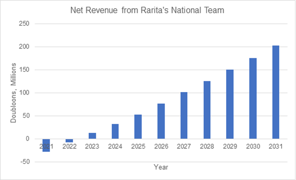
However, the initial reserve established for the team (995 million Doubloons) is sufficient to cover this outflow. As the team becomes competitive, revenue growth is expected to outpace that of expenses, with net revenues becoming positive in 2023 and thereafter. Thus, the team can generate positive returns and become a self-sustaining business model while achieving competitiveness, making the plan economically feasible at best estimate assumptions.
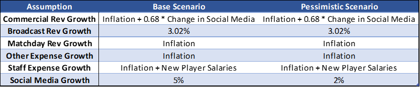
An alternative scenario was considered, changing our assumptions on the growth of social media presence for the Raritan national team to 2% p.a.
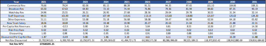
This yielded a lower result, but NPV of net revenues is still expected to be positive over the 10-year forecasting period.
Sensitivity Analysis
Base Social Media Growth Scenario
Sensitivity analysis was conducted on our base case revenue projections against changes in the growth rate of broadcast revenues, interest rates, and inflation.
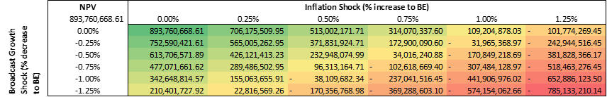
In the event of a 1.25% rise in annual inflation, the baseline estimate leads to a negative NPV regardless of changes in broadcast revenue growth.
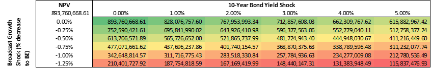
Interest rates and broadcast revenue growth appear less significant, with NPV projected as positive even with a 5% rise and -1.25% shock to both assumptions respectively.
Low Social Media Growth Scenario
Sensitivity tests were also conducted for a pessimistic scenario for social media growth (2% p.a. growth in social media).
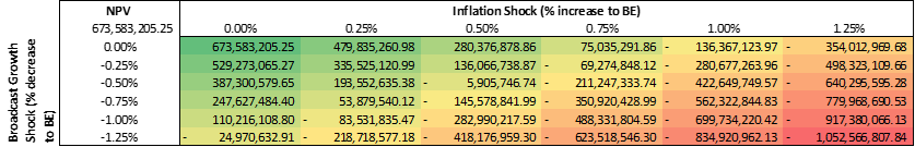
It can be observed that there is a significant increase in the number of scenarios that result in a negative NPV, with shocks to inflation upwards of 0.75% leading to negative NPV outcomes in almost all situations.
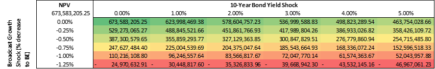
Like the base scenario, the variable which produces the greatest downside risk is inflation, with shocks to risk-free rates and growth of broadcast revenues still producing outcomes of positive NPV.
Managing Risks
From our sensitivity tests, the worst-case outcomes measured through the NPV are -785.13 million at 5% social media growth and -1052.57 million at 2% in the two scenarios. Thus, our initial funding of 995 million Doubloons should be sufficient to cover the potential losses in the majority of scenarios considered.
We advise the Raritan government to set up a reserve for 995 million and invest it at the 10-year treasury rate, allowing funds to be liquidated if assumptions materialise and are worse than expected. Although this strategy may expose the funds to interest-rate risk, this could be managed through hedging via instruments such as interest rate swaps and duration matching between assets and expected liabilities.
As noted previously, the external variable which poses the greatest threat on the strategy’s financing is inflation. To mitigate this risk, ongoing monitoring of the economic environment and inflation must be conducted. Cost-cutting measures and reducing staff expenses by constructing a less competitive team can be adopted as a last resort if economic conditions jeopardize the feasability of our proposed strategy. Allocating the initial reserves to assets such as inflation-linked bonds can also mitigate the potential imapacts of an inflationary shock on the revenues and expenses of the team.
Risks and Limitations

Through continual monitoring efforts as shown in our implementation timeline, key risks can be mitigated. These key risks include Rarita’s national team becoming uncompetitive, growth of competitors’ abilities, increased prices to loan players from external countries and inaccurate projections.
Furthermore, political risks can have negative implications on Rarita’s national team. The most notable consequence would be the prohibition of loaning external players which could reduce the competitiveness of Rarita’s team. However, the metric system designed would allow Rarita to quickly identify appropriate substitute players with constant monitoring to review the team’s performance.
In addition to risks, key limitations were also considered which are detailed in the table below.
| Limitation | Implication |
|---|---|
| Generating revenue by loaning Raritan players not included in net revenue | Revenues are understated but best estimates show they are sufficient |
| Only salaries of new players on national teams and inflation considered in expense projections | Currently no consideration for potential fixed costs (e.g. investment in infrastructure). These expenses must be included separately in the future if required |
| Team construction dependent on player data and metrics of competing teams, all of which only available for past periods | Opposing teams may improve significantly compared to previous years, which may our benchmarks for teambuilding irrelevant |
| Players are selected based on league statistics, so only players present in league dataset are considered in team selection | Some teams had a large number of players not present in league data and their team is unable to be evaluated by our metric. We also did not allow selection of non-league players in our team construction |
Conclusion
In conclusion, a competitive national team was constructed for Rarita using a metric developed from chosen statistics. The key objectives of achieving competitiveness were successfully met as Rarita’s national team is projected to continue improving and adapting to the future competition environment, espeically through the development of our player metric and continual monitoring. Overall, Rarita’s national team will build a brand for the country’s football program and achieve positive economic impacts for the country.
References
Brooks J., Kerr M., and Guttag J., 2016., Developing a Data-Driven Player Ranking in Soccer Using Predictive Model Weights, KDD ‘16: Proceedings of the 22nd ACM SIGKDD International Conference on Knowledge Discovery and Data Mining, pp. 49–55. DOI: 10.1145/2939672.2939695, Date Accessed: 15/03/2022
Ribeiro A. and Lima F., 2018, Football players’ career and wage profiles, Applied Economics, DOI: 10.1080/00036846.2018.1494375, Date Accessed: 15/03/2022
Stanojevic R. and Gyarmati L., “Towards Data-Driven Football Player Assessment,” 2016 IEEE 16th International Conference on Data Mining Workshops (ICDMW), 2016, pp. 167-172, DOI: 10.1109/ICDMW.2016.0031. Date Accessed: 16/03/2022